High-resolution population layouts

PyPSA-Spain provides a high-resolution variant of the build_population_layouts rule that uses Spanish municipality-level population data instead of the default NUTS3 aggregation.

The default PyPSA-Eur procedure overlays the cutout grid on NUTS3 region geometries, assumes population is homogeneously distributed within each NUTS3 region, and splits each grid cell into urban and rural fractions by sorting cells by density and cutting at a national urbanisation rate obtained from the World Bank. For Spain, this approach is coarse: NUTS3 regions correspond roughly to provinces, so the within-region homogeneity assumption masks the strong density contrast between cities and surrounding rural areas.

PyPSA-Spain replaces this procedure with a layout built directly from the ~8,100 Spanish municipalities. The urban share of the national population is set by the user via configuration, and the highest-density municipalities are tagged as urban until that share is reached.

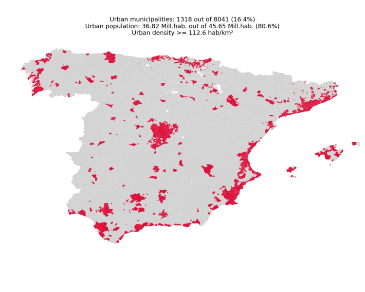
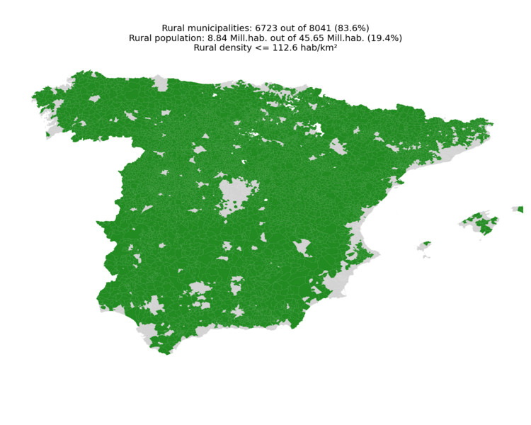
The following figures show the urban (left) and rural (right) classifications obtained with the default configuration (urban_fraction: 0.806):

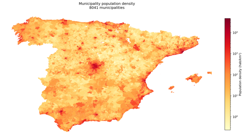
The choropleth of municipal population density (log scale) is shown below:

Data source and license

The municipality-level population dataset used by this functionality is published on Zenodo (record 20431328). It is a processed dataset derived from the demographic data released by the Spanish Ministry for the Ecological Transition and the Demographic Challenge (MITECO, Reto Demográfico — datos demográficos).

The processed dataset on Zenodo is released under the Creative Commons Attribution 4.0 International (CC BY 4.0) license. The original MITECO source data are reused under their own terms; see the original publisher’s legal notice for details.

Procedure

When the feature is enabled, the script overrides the three default pop_layout_{total,urban,rural}.nc files using the following steps:

1. Load the municipality boundary dataset (pop_ES_2023_LR.geojson, retrieved from Zenodo), which contains the resident population as of 1 January 2023 (pob_23) for each Spanish municipality.

2. Remove the municipalities of Canarias, Ceuta and Melilla before any subsequent calculation (see Modelling assumptions and limitations). All steps below operate on the resulting peninsular + Balearic subset.

3. Compute the population density of each remaining municipality as \(\rho_m = \text{pob2023}_m / A_m\), where \(A_m\) is the municipal area in km² computed in the ETRS89 / LAEA Europe projection (EPSG:3035).

4. Sort municipalities by density in descending order and tag the highest-density ones as urban until their cumulative population first reaches or exceeds the configured target urban fraction \(f_{\text{urban}}\) of the considered (peninsular + Balearic) population. The remaining municipalities are classified as rural. The boundary density (i.e. the lowest density still classified as urban) is reported in the log and shown as a horizontal line in the diagnostic step plot.

5. The script also logs, for reference, the World Bank urbanisation rate for Spain (used by the default PyPSA-Eur procedure) alongside the value taken from the configuration, so that the user can see how their choice compares to the official statistic.

6. For each cutout grid cell, distribute every municipality’s population homogeneously across its area and accumulate the contributions intersecting the cell. This is computed via the atlite indicator matrix:

   \[p^{\text{cell}}_i = \sum_m \frac{A(c_i \cap m)}{A_m} \cdot \text{pob2023}_m\]

   The same expression yields pop_layout_total, pop_layout_urban and pop_layout_rural by summing over all, only urban, or only rural municipalities respectively. Following the convention of the default NUTS3 flow, the resulting NetCDF layouts store values in thousands of inhabitants (pob2023_m is divided by 1000 before accumulation).

The three NetCDF files are then overwritten with the new layouts.

In addition, the urban and rural municipalities are exported as two CSV files (municipalities_urban.csv and municipalities_rural.csv) under resources/{PREFIX}/{NAME}/pop/. Each row stores the unique INE code (codmun_ine), name (nombre), autonomous community (ccaa) and population (pob_23) of one municipality, providing a single source of truth for the urban/rural classification that downstream rules can reuse without re-running it.

Per-region aggregation

The default PyPSA-Eur build_clustered_population_layouts rule aggregates the cell-level layouts to the clustered model regions using an indicator matrix \(I[r, c] = A(c \cap r) / A(c)\), which implicitly assumes that population is uniformly distributed over the entire cell. For coastal cells this is a poor assumption: population is concentrated in the onshore sliver covered by municipalities, while the rest of the cell lies offshore and is also outside the onshore region. As a result, part of the population deposited on those slivers is silently dropped and the per-region totals fall short of the cell-level totals.

When pop_layouts_HR.enable is active, PyPSA-Spain bypasses the cell intermediation in build_clustered_population_layouts: it loads the urban / rural classification from the two CSV files, retrieves each municipality’s geometry from the original GeoJSON (joined by codmun_ine), and aggregates populations to clustered regions through an area-weighted indicator matrix

\[M[r, m] = \frac{A(r \cap m)}{A(m)}, \qquad p^{\text{region}}_r = \sum_m M[r, m] \cdot p^{\text{muni}}_m\]

Each municipality’s population is split across the regions that intersect it in proportion to area overlap, so total population is preserved exactly for fully-covered municipalities (i.e. all peninsular and Balearic municipalities once Canarias, Ceuta and Melilla are excluded). The fraction of municipal area falling outside regions_onshore and the corresponding lost population are reported in the log as a diagnostic.

Configuration

The functionality is enabled in the pypsa_spain module of config/config_ES.yaml:

pop_layouts_HR:
  enable: true
  file: data_ES/pop/2023/pop_ES_2023_LR.geojson
  urban_fraction: 0.806

The urban_fraction parameter sets the target share of the national population to be classified as urban (e.g. 0.806 means that the 80.6% of the population living in the highest-density municipalities is treated as urban).

When enable: false, the script falls back to the default NUTS3-based PyPSA-Eur layouts and the input shapefile is not required.

Diagnostic plots

When the feature is active, the rule also produces four diagnostic figures under resources/{PREFIX}/{NAME}/pop/:

• map_urban.png — map of all municipalities, with urban ones (density above the threshold) coloured. The title reports the number of urban municipalities and the share of national population they account for.

• map_rural.png — analogous map highlighting rural municipalities.

• map_density.png — choropleth of municipal population density, plotted on a logarithmic colour scale.

• density_steps.png — descending step plot of municipal density. Each step has height equal to the municipality’s density and width equal to its population, so cumulative width on the x-axis equals the cumulative population from highest- to lowest-density municipalities. A horizontal red line marks the boundary density that delimits the configured urban fraction; the title shows the resulting urban / rural population split.

Modelling assumptions and limitations

• Population is assumed to be homogeneously distributed within each municipality.

• Only Spanish municipalities are covered. If the cutout extends beyond Spain, grid cells outside the municipal coverage receive zero population in all three layouts.

• Municipalities in Canarias, Ceuta and Melilla are excluded from the high-resolution layout, since they fall outside the cutout footprint used for the modelled system. Their population is therefore not represented in the per-cell or per-region outputs when the high-resolution mode is active.